Avances en Psicología Latinoamericana
ISSN:1794-4724 | eISSN:2145-4515

Introduction

Over time, the tripartite conception of validity (content validity, criterial validity and construct validity) has evolved into the current unified conception in which construct validity represents a fundamental aspect (Messick, 1994; Smith, 2005).

The construct validation process includes a set of actions, among which the study of the internal test structure is often highlighted. In this sense, it is usually devoted much effort to obtain empirical data in order to know the kind of relation set between the hypothesized variables and the scores through measurement instruments (Shadish, Cook & Campbell, 2002). Factor analysis plays a central role, since it is the most applied method to obtain evidences about construct validity because it provides information about the internal structure of the measurement instrument (Zumbo, 2007).

When using Confirmatory Factor Analysis —CFA—, certain requirements must be met: adequate sample size, random sample collection, independent observations, multivariate normality of observed variables, absence of collinearity, linearity, additivity of effects and the fact that both latent and that observed variables are continuous (Mulaik, 1972). However, most of these assumptions contradict the nature of the data which are usually obtained in Social Sciences through Likerttype questionnaires, where the latent construct is continuous in nature while the observed variables are measured according to an ordinal scale (Coenders & Saris, 1995; DiStefano, 2002; Finney, DiStefano & Kopp, 2016; Flora & Curran, 2004; Freiberg, Stover, De la Iglesia & Fernandez, 2013). Consequently, one of the requirements for using CFA is not fulfilled, that is, the continuous nature of both latent and observed variables.

Despite this lack of fulfilment, treating observed variables as if they were continuous has been usual. In this sense, most of studies apply Maximum Likelihood —ML— method in the CFA phase of parameter estimation (Brown, 2006). Apart from homocedasticity and residual independence, the ML assumes both normal distribution and continuous nature of observed variables (Bollen, 1989). It is an estimation method based on a Pearson correlation matrix, since it is assumed that observed variables correspond to an interval scale (Coenders & Saris, 1995).

O’Brien (1985) has analysed the problems related to the use of Pearson correlations in Likert-type scales. Among them, we can remark the variability reduction of the observed variables, whereby it is registered a lower correlation between them (Saris, Van Wijk & Scherpenzeel, 1998; DiStefano, 2002; Holgado-Tello, Chacón-Moscoso, Barbero-García & Vila-Abad, 2010). This fact, in turn, reduces the relationship between latent constructs and observed variables. Jöreskog and Sörbom (1996a, 1996b) propose using polychoric correlations to know the degree of correlation between ordinal variables. Polychoric correlations are an alternative which helps to overcome the problems associated with Pearson correlations (Coenders & Saris, 1995; Holgado-Tello et al., 2010; Choi, Peters & Mueller, 2010).

The multivariate normal distribution of observed variables is another aspect which also fails, in this case occasionally, in the fulfilment of CFA requirements (Flora & Curran, 2004). It seems that items’ skewness is one of the main causes (Coenders & Saris, 1995). While using the ML method requires that the observed variables follow the normal distribution, some researchers, such as Boomsma and Hoogland (2001), and Muthén and Muthén (2002), state that this method is robust to the failure to meet this assumption. For its part, Kaplan (1990) considers that ML can be used when the univariate skewness is lower than 1 in all the variables which are part of the analysis.

It is worth recalling that model building in CFA consists of different stages. First of all, the model is specified and identified. After collecting data, model parameters are estimated. Then the model fit is evaluated. One of the CFA fundamental aspects focuses on the model estimation phase. In few words, in this stage the generic expression F = [ S - Σ (p) ]’ W [ S - Σ (p) ] is minimized (Bollen, 1989). On the one hand, in this adjustment function, [S - Σ (p)] the residual matrix is obtained after calculating the difference between two variance- covariance matrices: S from the sample and Σ (p) from the model parameters. On the other hand, W is the weighing matrix.

According to Jöreskog and Sörbom (1988), from an asymptotic covariance —AC— matrix a freely distributed weighing matrix W is obtained, which is involved in the adjustment function of the Robust Maximum Likelihood method or RML (Bentler, 2006; Jöreskog & Sörbom, 1996b), the Weighted Least Squares method or WLS, and the Robust Unweighted Least Squares method or RULS (Yang-Wallentin, Jöreskog & Luo, 2010). These estimation methods are an alternative to the ML method. More specifically, when continuous observed data do not follow the normal distribution it is advisable to use an asymptotically distribution- free method: WLS (Brown, 2006; Yang-Wallentin et al., 2010). If any of the observed variables is categorically measured, the WLS method allows the use of polychoric correlations (Jöreskog & Sörbom, 1989). It is worthy to mention —and it is the main limitation of this method— that the model must not have neither over 10 variables nor a moderate sample size, that is, less than 1000 cases (Satorra, 1990). For small or medium-sized samples the RML method has shown a better performance than WLS (Curran, West, & Finch, 1996; Hu & Bentler, 1992). The RML method, as in the case of the WLS, can be applied when observed variables are continuous in nature and data do not follow the normal distribution, although RML provides the Satorra-Bentler χ2 statistic (Brown, 2006; Finney & DiStefano, 2006). As regards the ULS method, it does not establish a certain distribution of categorical observed variables (Bollen, 1989; Brown, 2006; MacCallum, 2009). Finally, the RULS method, analysed by Yang-Wallentin et al. (2010), is a robust variant of ULS because both of them work with a polychoric correlations matrix, but, when using RULS, this kind of correlation is the basis for obtaining the AC matrix thereafter, which is involved in a freely distributed weighing W matrix, since observed variables do not fulfil the multivariate normal distribution assumption.

It is important to note that, as far as we know, both the RML and the RULS methods have been used by a minority of recent studies. Although these estimation methods begin to be used more frequently in applied research, simulation studies focused on Type I error and power of parameter estimation methods are still scarce. To mention a few, we should highlight the studies done by Lei (2009), Holgado-Tello, Morata-Ramírez and Barbero-García (2016), Sass, Schmitt and Marsh (2014), Savalei and Rhemtulla (2013), and Yang-Wallentin et al. (2010).

Briefly, in studies about statistical power, Bollen (1989) identifies two basic principles: (1) the positive relationship between Type I error and the statistical power of a test, and (2) the power dependence upon the specific value of a parameter under the alternative hypothesis. At the same time, although the statistical power increases as a sample size does, there are other features involved in power level (Saris & Satorra, 1988). Through the χ2 likelihood ratio test parameters can be detected that must be added to the theoretical model. Thus, the power of the test corresponds to the probability of detecting specification errors, for either a lack of a sufficient number of parameters or the setting of incorrect constraints in the model.

One of χ2 statistic limitations related with the present study has to be pointed out: its sample size sensitivity, which results in a slight trend to the rejection of probably correct theoretical models with a big sample size (Hu & Bentler, 1995). Despite this, the alternative goodness of fit indices does not allow to set a clear relationship between the fit index and the model specification errors (Saris & Satorra, 1993).

The rejection of the null hypothesis associated to low power has often been interpreted as an evidence of serious misspecification. Additionally, if the likelihood ratio test determines a good fit and simultaneously the power is high, it is considered that there are no serious specification errors. At this point, it has to be taken into account that Saris and Stronkhorst (1984) warn about the insignificant specification errors related to the rejection of null hypothesis when the power is high, whereas maintaining the null hypothesis when the power is low might hide undetected serious specification errors, which seriously affect the evidences for obtaining construct validation.

Finally, it must be noted that the AC matrix is not only involved in certain parameter estimation methods to apply when the observed variables are measured according to an ordinal scale. As we will see, this matrix is also present when analysing goodness of fit using the χ2 likelihood ratio test. According to Jöreskog (2004), the AC matrix is necessary to obtain the χ2 statistic if the observed variables do not fulfil the multivariate normality assumption, and consequently different χ2 values are obtained: C1 (“Minimum Fit Function Chi- Square”), C2 (“Normal Theory Weighted Least Squares Chi-Square”), C3 (“Satorra-Bentler Scaled Chi-Square”) and C4 (“Chi-Square Corrected for Non-Normality”).

In connection therewith, χ2 values depend on the parameter estimation method previously used. When the multivariate normality assumption is fulfilled, C1 and C2 indices are obtained for ML method and C1 index for ULS method, whereas, when that assumption is not fulfilled, AC matrix allows to obtain C1, C2, C3 and C4 indices for the RML method and C1 index for the WLS method (Jöreskog, 2004). Following this pattern, C2, C3 y C4 indices are obtained for the RULS method.

To sum up, an important point to remember when using factor analysis to check construct validity is the measurement scale of the instrument (Flora, Finkel & Foshee, 2003). In addition, Shadish et al. (2002) as well as Flora and Curran (2004) consider that the conclusions derived from empirical data about a theoretical model can be affected by the mismatch between what the statistical model assumes and the characteristics of the analysed data. Since it is necessary that the theoretical models reproduce the relationships between the variables of a construct as faithfully as possible, there should be consistency between the estimation methods and the measurement instrument. Given the existing estimation methods and data characteristics, the objective of the present simulation study is to analyse the influence of a set of experimental factors (number of factors, number of response categories, items’ skewness, and sample size) on Type I error and power related to different estimation methods. Specifically, five estimation methods are compared: ML, RML, WLS, ULS, and RULS.

Method

Four experimental factors were manipulated: a) number of factors, or latent variables, b) number of response categories, c) items’ skewness, and d) sample size. The number of factors had five levels (2, 3, 4, 5 and 6). For each factor three items were simulated. The factor loadings of the items were always the same in all factors, namely 0.9, 0.8 and 0.7 for the first, second and third item of each factor. The simulated factor loadings were high in order to avoid doubts about the specification in the parameters estimation stage. Items were generated according to a normal distribution N(0,1). Then, these answers were categorized according to 3, 4, 5, and 6 points Likert-type scales. These scales were categorized so that: a) the responses to all items remained symmetrical, b) all items had moderate skewness, or c) all items had severe skewness. Thus, items’ skewness had three experimental levels: skewness = 0; skewness = 1, or moderate; skewness = 2, or severe.

To categorize Likert-type scales, as stated by Bollen and Barb (1981), the continuum was divided into equal intervals from z = -3 to z = 3 in order to calculate the thresholds of the condition in which the response distribution to all items is symmetrical (skewness = 0). For skewed distributions, the thresholds were calculated, according to Muthén and Kaplan (1985), in a way that observations were accumulated in one of the extreme categories as the degree of skewness increased. Half of the variables of each factor were categorized with the same positive skewness and the rest of variables with the same negative skewness with the purpose of simulating difficulty factors. Finally, sample size had six experimental values (100, 150, 250, 450, 650 and 850 cases).

The combination of the four experimental factors (number of factors, number of response categories, items’ skewness and sample size) produced 360 experimental conditions (5 x 4 x 3 x 6) which were replicated 500 times. These replications were performed using R version 2.12.0, which invoked successively Prelis version 2.0 to generate the corresponding data matrices according to the specifications resulting from the combination of the experimental conditions. Thus, for each generated matrix, we obtained Pearson and polychoric correlations matrices as well as asymptotic covariance matrices.

After obtaining correlations matrices and asymptotic covariance matrices for each data matrix generated under the concrete specifications of the experimental factors, we conducted the corresponding Confirmatory Factor Analysis (CFA) successively, that is, until 500 times (one CFA for each replication). As in the previous case, these replications were performed using R version 2.12.0, which invoked successively LISREL version 8.8. There were two types of theoretical models which were tested through LISREL: (1) correctly specified models: this means that the specified theoretical model using LISREL syntax corresponds exactly with the model which has enabled data generation, and (2) misspecified models: in this case the theoretical model specified using LISREL syntax does not correspond exactly with the model that has enabled data generation. To do this, the syntax specifies a model so that an item of each factor saturates incorrectly in another one.

The combination of these criteria produced 360 000 replications (180 000 for correctly specified models and the same amount for misspecified models) for each estimation method. Taking into account the five estimation methods, a total of 1 800 000 (5*360 000) replications were generated.

In order to facilitate the management and compilation of fit indices files, a specific program was generated in Java language.

Data Analysis

Type I error was the percentage of rejections of the null hypothesis in correctly specified models. Power (1-β) was the rejection percentage of the null hypothesis in misspecified models. We made these calculations for each of the χ2 values reported in the LISREL output files obtained for each estimation method used in the present study. The χ2 values obtained for each estimation method, depending on the fulfilment of the multivariable normality assumption, were the following ones: C1 and C2 for the ML method; C1, C2, C3 and C4 for RML; C1 for WLS; C2 for ULS; and finally C2, C3 and C4 for RULS. We used a probability of 0.05 as significance level.

Results

In the lines below, it must be taken into consideration that there were some experimental conditions for which it was not possible to obtain results, due to the fact that, as we mentioned in the introduction, the use of the WLS method requires the fulfilment of certain conditions. In this regard, when the responses to all items had a symmetrical distribution, there were no available results, regardless of the number of categories, for models with 5 factors and 100 cases and for models with 6 factors and 100 or 150 cases. When the responses had a moderate skewed distribution, there were no available results, irrespective of the number of categories, for models with 5 or 6 factors and 100 cases and for models with 6 factors and 100 or 150 cases. There were also no results for models with 5 factors, 3 response categories and 150 cases, as well as both for models with 6 factors, 3 response categories and any of the remaining sample sizes analysed and for models with 6 factors, 5 response categories and 850 cases. When the responses had a severe skewed distribution, there were no results, independently of the number of categories, for models with 5 factors and 100 cases and for models with 6 factors and 100 or 150 cases. For this reason, the findings about WLS must be cautiously considered when this method is compared with the others.

Influence of the Number of Factors

Table 1 displays the results about Type I error and power of each of the estimation methods depending on the number of factors of the theoretical models examined.

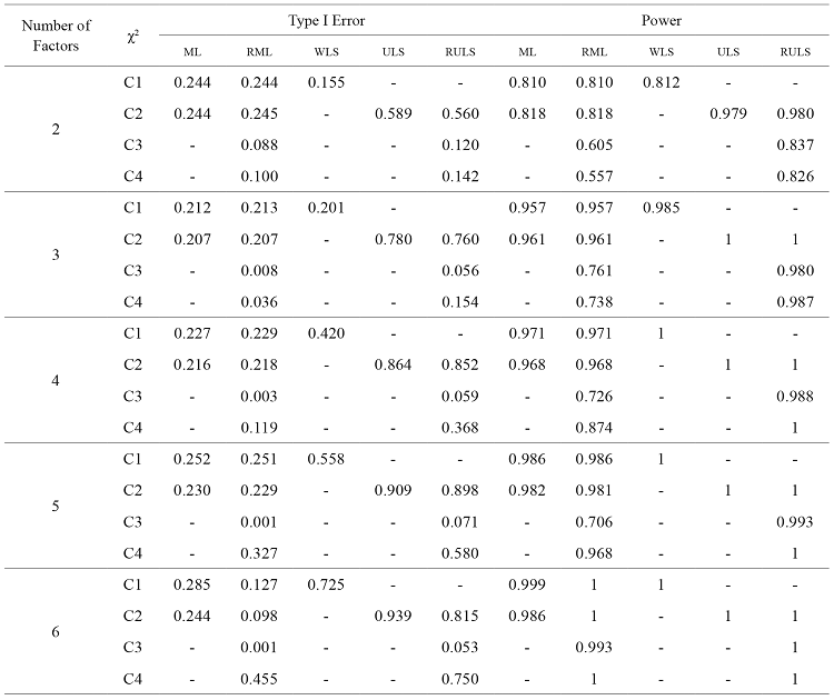
With regard to the ML, Type I error values are quite alike, regardless of the number of factors of the model. In fact, Type I error is mostly above 0.22 although it presents the lowest value for models with three factors (0.207). For its part, power is slightly greater as the number of factors increases. Thus, the power is .818 in models with two factors, whereas it is 0.986 in models with six factors. In other words, as the number of factors increases, the probability of accepting a false model is lower.

In the RML method Type I error decreases as the number of factors of the model increases. In fact, when the model has two factors, Type I error is 0.088, and when the model has five or six factors, this value is 0.001. Power presents an increasing pattern as the number of factors goes from two to three (0.605 and 0.761, respectively). Then, its values are similar to some degree but they increase when the factors of the model rise from five to six (0.706 and 0.993, respectively). Consequently, the probability of accepting a false model decreases as a model takes more factors into account.

As regards the WLS, Type I error is higher as the models have more factors. This value is 0.155 in models with two factors and raises to 0.725 in models with six factors. Apart from that, power improves as the dimensions of the evaluated models increase and it shows the maximum value from four factors on.

The ULS method follows the same pattern as the WLS, that is to say, as the number of factors increase, Type I error and power also increase. In this case, power reaches the maximum value for models with three or more factors.

For the RULS we find a similar trend to the one shown by the RML method. Thus, as the number of factors increases, Type I error improves, since in models with two factors Type I error is 0.120, and in models with six factors it is 0.053 (around the nominal value of the significance level of 95 %, which is taken as a reference). For their part, power values approach progressively to 1 as the number of factors approximates to six.

Comparing the results, robust estimation methods show the lowest Type I error and the highest power. Both methods show higher Type I error percentages for two factors models, but the values are lower for the RML method, regardless of the number of factors. As regards power, these methods display an improvement as long as the dimensions of the models increase, although power is higher with the RULS method rather than with RML, particularly for models with few factors.

Concerning non-robust methods, Type I error of ML is quite similar, independently of the number of factors, whereas power improves slightly as the number of factors increases. In addition, when using the WLS method, as the number of factors increases, Type I error worsen but power improves. The ULS method displays a similar trend, and it is worthy to remark that it shows the highest percentages of Type I error and power with respect to the remaining estimation methods analysed.

Influence of the Number of Categories

In table 2 we present the results related to the number of categories.

With respect to the ML method, Type I error values are pretty similar, regardless of the number of categories. In this context, models with three response categories show the lowest Type I error (0.200), whereas models with four response categories display the highest one (0.267). Power values are close to each other, irrespective of the number of categories, but they are greater for models with four categories (0.956).

As regards the RML, Type I error tends to be similar over the number of response categories, albeit for models with four categories it is markedly higher (0.069) than the rest. Power is mostly rather alike as the number of categories increases, although models with three categories display a lower one (0.600).

The WLS method, like both ML and RML, shows a quite similar Type I error, regardless of the number of categories, but models with four categories display a noticeable higher Type I error (0.452). Power is pretty alike all over the number of categories, but it shows a greater value for models with four categories (0.970).

With respect to the ULS method, Type I error decreases as the number of categories increases. Thus, in models with three categories, the Type I error is 0.926, whereas in models with six categories it is 0.705. In other words, as models have a higher number of categories, the probability of rejecting a correctly specified model is lower. Power values almost reach the maximum value irrespective of the number of categories.

As regards the RULS, Type I error is rather similar in relation to the number of categories, even though it is clearly greater when the model has four response categories (0.120). In case the evaluated model has five or six response categories, the Type I error values are respectively 0.058 and 0.054, namely close to 0.05 (the nominal value of 95 % significance level). For its part, power is mostly pretty alike over the number of categories. In fact, models with three categories show their lowest value (0.939).

Comparing the estimation methods amongst each other, ML, RML, WLS and RULS coincide with the fact that a Type I error is more likely to occur when models have four response categories. Besides, these methods show individually pretty similar power values, except for models with three or four categories, which are more or less noticeably higher than the rest of categories.

As we mentioned before in relation to the number of factors, Type I error values in robust methods are the lowest ones and power values are the highest ones. Albeit both robust methods show a higher Type I error for models with four response categories, it is also true that the RML shows lower values than the RULS, regardless of the number of categories. In addition, the RULS Type I error is close to the nominal value of the significance level of 95 % for reference purposes if the evaluated model has five or six response categories. In relation to power, the RULS displays higher values than the RML as the number of categories is small as well as for the number of factors.

As far as the ULS is concerned, when the number of categories grows, the Type I error decreases and its power reaches very near to the maximum value whatever the number of categories. It is worthy to note that both ULS Type I error and power are once again the highest in comparison with the remaining estimation methods.

Influence of the Items’ Skewness

Table 3 shows the results related to items’ skewness.

As regards the ML, the Type I error increases as the skewness of the responses distribution does. Thus, when the distribution is symmetrical, the Type I error is 0.054 (around the nominal value of the significance level of 95 %), whereas when the distribution has a severe skewness, the Type I error is 0.476. In other words, as skewness grows, it is more probable to reject a correctly specified model. In addition, power decreases as the responses distribution is more skewed. Namely, power is 0.978 in models with a symmetrical responses distribution, and it descends until 0.897 for models whose distribution has a severe skewness. Therefore, as the degree of asymmetry increases, it is more likely to accept a false model.

For its part, the RML shows that the Type I error grows as the response distribution changes from symmetrical to moderate skewed. However, Type I error values are alike in case the skewness is moderate or severe. In fact, when the responses distribution is symmetrical, the Type I error is 0.006, whereas, when the distribution has a moderate or a severe skewness, this value is 0.034 and 0.033, respectively. For its part, power decreases in a noticeable way. That is, for symmetrical distribution the power is 0.941, whereas it is 0.737 and 0.436 in models whose response distributions have moderate and severe skewness, respectively.

When the WLS is applied, the Type I error shows similar values when the responses distribution is symmetrical or has a moderate skewness, but it slightly increases if the distribution has a severe skewness. In fact, when the distribution is symmetrical, the Type I error is 0.371, when the response distribution has a moderate asymmetry, the Type I error is lower (0.358), and when with a severe skewness, the Type I error is 0.412; that is, higher than symmetrical distributions. For its part, power is slightly lower as the skewness of the responses distribution grows, going from 0.968 to 0.940 for models with a symmetrical and a severe skewed distribution, respectively.

For the ULS, the Type I error increases as the degree of skewness of the responses distribution does. In fact, when the distribution is symmetrical, the Type I error is 0.573, whereas when it has a moderate or a severe skewness this value is 0.900 and 0.975, respectively. In other words, as the degree of skewness grows, it is more likely to reject a correctly specified model. Power values are almost 1, regardless the degree of skewness.

Regarding the RULS with respect to the Type I error, it is higher as the response distribution goes from being symmetrical to have a moderate skewness, whereas it displays similar values when the response distribution has a moderate or a severe skewness, like the RML. In fact, when the distribution is symmetrical, Type I error is 0.054 (around the nominal value of the significance level of 95 %, which is taken as a reference), whereas, when the distribution has a moderate or a severe skewness, this value is 0.092 and 0.086, respectively. Apart from that, power decreases in accord with the increasing of skewness in the responses distribution. In fact, in models with a symmetrical distribution, power has a value of 0.977 and it falls to 0.919 when the skewness is severe. That is to say, as the degree of skewness grows, it is more likely to accept a false model.

Comparing the estimation methods analysed in the present study each other, RML and RULS show a similar pattern in the Type I error and power values as the responses distribution is more skewed. In this sense, the passage from a symmetrical distribution to a moderate skewed distribution represents an increase of Type I error, and then for moderate or severe skewed distributions Type I error values are very alike. In addition, power for both RML and RULS worsens as the degree of skewness grows, particularly for RML.

As regards non-robust estimation methods, the Type I error for WLS displays pretty similar values in both symmetrical and moderate skewed distributions, but this value increases when the distribution has a severe skewness. For its part, the WLS power follows a light downward tendency. In addition, Type I error and power for the ML method decrease as the skewness of the responses distribution is greater. The ULS method shows again the highest Type I error values among the estimation methods analysed, whereas power almost reaches the maximum value for any of the skewness degrees considered.

Influence of the Sample Size

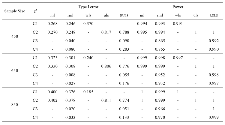
In table 4 we show the results about Type I error and power for each of the estimation methods depending on sample size of theoretical models.

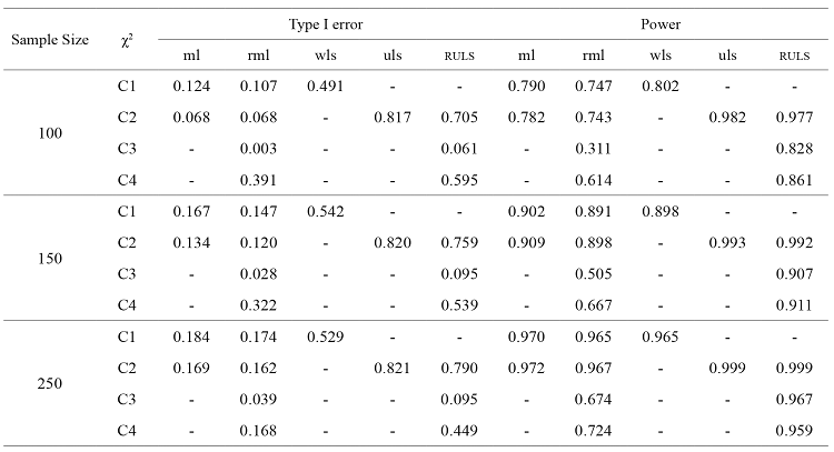
When the ML method is used, the Type I error increases as sample size grows. Thus, in models with 100 cases the Type I error is 0.068, whereas in models with 850 cases this value is 0.402. In other words, as the number of cases increases, it is more likely to reject a correctly specified model. On the contrary, power improves when the sample size is greater. In this sense, in models with 850 cases it reaches the maximum value, though the power of models with 450 and 650 cases is already almost 1.

For the RML, Type I error values are quite alike in relation to the sample sizes considered in the present study. However, sample sizes of 100 and 650 cases display the lowest Type I error, since its values are 0.003 and 0.008, respectively. Power increases as sample size does. That is to say, as sample size is smaller, the probability of accepting a false model is greater.

As regards the WLS method, the Type I error shows similar values when the sample size is between 100 and 250 cases. Therefore, in models with 100 cases the Type I error is 0.491, whereas in models with 250 cases this value is 0.529. For its part, a noticeable downward trend in Type I error is observed when the sample size of models goes from 450 to 850 cases. In fact, in models with 450 cases the Type I error is 0.370, whereas in models with 850 cases this value is 0.185. On the contrary, power improves as sample size increases, and in models with 850 cases the power is 1. However, the power of models with 450 and 650 cases almost reaches the maximum value.

With respect to the ULS, Type I error values are pretty similar regardless of the sample size of models. In fact, when models have 100 cases, the Type I error is 0.817, and this value is 0.811 for models with 850 cases. For its part, the power improves as the sample size grows, and it shows the maximum value in models whose samples are equal to or over 450 cases, even though its values are almost 1 for models with 150 and 250 cases.

When using the RULS, the Type I error is close to 0.050 (around the nominal value of 95 % significance level) when models have 100, 650 and 850 cases, whereas for the remaining sample sizes (that is, 150, 250 and 450 cases) Type I error is around 0.090. Therefore, there is an upward trend in Type I error when sample sizes go from 100 to 150 cases, and a downward trend when models have 650 and 850 cases. Power improves as the sample size increases. Thus, in models with samples sizes with 850 cases its value is maximum, although models with 450 and 650 cases display power values which are almost 1.

Comparing the estimation methods for each other, for the ML the Type I error increases as sample size is bigger, whereas it decreases for WLS. Power is higher as the sample size is greater. For both methods, models with 850 cases show the maximum power, even though the power of sample sizes with 450 and 650 cases is already very close to 1. As far as ULS is concerned, the Type I error and power values are again the highest in comparison to the rest of the estimation methods analysed. Besides, the ULS method displays the maximum value for samples equal to or over 450 cases, although the power of samples with 150 and 250 cases is almost 1.

Regarding robust estimation methods, for both RML and RULS the Type I error is quite similar, irrespective of sample size. Specifically, its values for the RML are once again lower than for the RULS. In relation to power, the RULS shows higher values than RML as for the previous experimental conditions.

Discussion

Number of Factors

Taking into account the number of factors of the models analysed, while the ULS method displays the highest rejection of misspecified models percentages according to power results, it is also true that its Type I error values imply the highest rejection of correctly specified models. With respect to robust estimation methods, they show a lower Type I error than the ML and WLS, although the Type I error with the ruls method is slightly higher than with the RML. Power results with the RULS are at higher levels than RML, and there are more noticeable differences between both methods when there are fewer factors.

Number of Categories

When we examine Type I error and power results related to the number of categories of the models, the ULS is the estimation method where the highest power and the Type I error coincide. Consequently, this method gives rise to the rejection of a larger amount of correctly specified models than other methods. Leaving aside the ULS, the robust methods display the lowest Type I error. Particularly, the RML shows a lower percentage of correctly specified models rejection in comparison to the RULS, but the RULS shows power values close to the maximum, irrespective of the number of categories. Besides, power differences between RML and RULS are more evident as there is a less number of categories.

Items’ Skewness

In terms of the skewness’ degree of the responses distribution, the ULS method is the one that shows one more time the highest percentages of rejection of misspecified models, but at the same time it rejects the highest amount of correctly specified models, especially those with a moderate or severe skewed distribution. Regarding the rest of methods, both RML and RULS display again the lowest Type I error. It is lower for the RML, which remains at the same percentage for moderate and severe skewness levels. With reference to power, as skewness grows, the RML method displays a lower percentage of rejection of misspecified models than RULS does. Additionally, power for RML decreases noticeably as skewness grows. Thus, the RULS method appears to be the most beneficial.

Sample Size

Concerning sample size, power percentages obtained with the ULS method are the highest ones in comparison to the rest of estimation methods, regardless of the number of cases of the models. However, the Type I error is also the highest one for the ULS, so it rejects the most important amount of correctly specified models. In terms of the other estimation methods, RML and RULS display the lowest Type I error, although RML percentages are even lower than those of RULS. Power obtained with the RULS is higher than with the RML for any sample size. Hence, using the RULS seems to be the best, particularly for models with 100, 650 and 850 cases, whose Type I error is smaller and close to the nominal level (0.050).

Comparison between Methods and General Guidelines

The results indicate that the RULS estimation method is more advantageous than any of the remaining methods analysed. In this sense, compared to ML, RML, WLS and ULS, using the RULS method reduce the probability of rejecting correct specified models and increase the probability of rejecting misspecified models taking into account the number of factors, the number of categories, items’ skewness, and sample size separately. This outcome is in line with Jöreskog and Sörbom (1989), who defend estimation methods which use polychoric correlations when dealing with Likert-type scales. In this regard, according to Jöreskog and Sörbom (1988), considering that ordinal variables are measured on an interval scale provides distorted parameters estimations and incorrect χ2 goodness of fit values.

Considering globally the results, the RULS, comparing to the others methods, seem to be a estimation method that works adequately, independently of the factors manipulated.

Limitations of the Study and Suggestions for Future Research Lines

In this paper, we present obtained results which can only be applied for misspecified models whose features correspond to the same number of factors, number of categories, items’ skewness and sample size. It would be interesting in future research to expand the range of misspecified models, taking into consideration contributions such as Sharma, Mukherjee, Kumar and Dillon (2005) in the sense that they include in their study up to 12 types of models according to their degree of misspecification.

When stablishing non-normality levels, not only skewness degree but kurtosis should have been taken into account, as Flora and Curran (2004) do. These authors point out that the WLS method implies the calculation of fourth order moments, and consequently kurtosis is involved in the results obtained. Additionally, Bentler (2006) warns about the multivariate kurtosis (MK) influence on RML results, since a MK lower than 5 advises not to apply the RML method (Yang & Liang, 2013).

Concerning sample size, when using the WLS method there were non-positive definite matrices due to an insufficient number of cases. Future studies should include experimental conditions with sample sizes greater than 850 cases.

Given the limitations of the χ2 likelihood ratio test, namely its sensitivity to sample size and its underlying assumption whereby a good fit of the model in the population means a perfect fit (instead of, as it actually occurs, an approximate fit), it is advisable that conclusions from its results are complemented with other goodness of fit indices. Consequently, in future research it might be interesting to study the information that provide other goodness of fit indices related to the characteristics of the theoretical models. In addition, aspects not considered in this paper, such as the item number per dimension (that was not included because the complexity of the theoretical models could affect the results), or the significance level, should be analysed in forthcoming researches.

References

Author notes

* Main contact for editorial correspondence purposes Francisco Pablo Holgado-Tello, Email: pfholgado@psi.uned.es

References

Bentler, P. M. (2006). EQS 6 structural equations program manual. Encino: Multivariate Software Inc. Retrieved from http://www.econ.upf.edu/~satorra/CourseSEMVienna2010/EQSManual.pdf
Bollen, K. A. (1989). Structural equations with latent variables. New York: Wiley.
Bollen, K. A. & Barb, K. H. (1981). Pearson’s r and coarsely categorized measures. American Sociological Review, 46(2), 232-239. DOI: 10.2307/2094981
Boomsma, A. & Hoogland, J. J. (2001). The robustness of lisrel modeling revisited. In R. Cudeck, S. du Toit & D. Sörbom (eds.), Structural equation models: Present and future. A festschrift in honor of Karl Jöreskog (pp. 139-168). Chicago: Scientific Software International.
Brown, T. A. (2006). Confirmatory factor analysis for applied research. New York: Guildford Press.
Choi, J., Peters, M. & Mueller, R. O. (2010). Correlational analysis of ordinal data: From Pearson’s r to Bayesian polychoric correlation. Asia Pacific Education Review, 11, 459-466. DOI: 10.1007/s12564-010-9096-y
Coenders, G., & Saris, W. E. (1995). Categorization and measurement quality. The choice between Pearson and Polychoric correlations. In W. E. Saris & Á. Münnich (eds.), The Multitrait-Multimethod approach to evaluate measurement instruments (pp. 125-144). Budapest: Eötvös University Press.
Curran, P. J., West, S. G. & Finch, G. F. (1996). The robustness of test statistics to nonnormality and specification error in confirmatory factor analysis. Psychological Methods, 1, 16-29. DOI: 10.1037/1082-989X.1.1.16
DiStefano, C. (2002). The impact of categorization with confirmatory factor analysis. Structural Equation Modeling, 9(3), 327-346. DOI: 10.1207/S15328007SEM0903_2
Finney, S. J. & DiStefano, C. (2006) Non-normal and categorical data in structural equation modelling. In G. R. Hancock, & R. O. Mueller (eds.), Structural Equation Modelling: A second course (pp. 269-314). Greenwich: Information Age Publishing.
Finney, S., DiStefano, C. & Kopp, J. (2016). Overview of estimation methods and preconditions for their application with structural equation modeling. In K. Schweizer, & C. DiStefano (eds.), Principles and methods of test construction: Standards and recent advancements (pp. 135-165). Boston: Hogrefe.
Flora, D. B. & Curran, P. J. (2004). An empirical evaluation of alternative methods of estimation for confirmatory factor analysis with ordinal data. Psychological Methods, 9(4), 466-491. DOI: 10.1037/1082-989X.9.4.466
Flora, B. F., Finkel, E. J. & Foshee, V. A. (2003). Higher order factor structure of a self-control test: evidence from confirmatory factor analysis with polychoric correlations. Educational Psychological Measurement, 63(1), 112-127. DOI: 10.1177/0013164402239320
Freiberg, A., Stover, J.A., De la Iglesia, G. & Fernández, M. (2013). Correlaciones policóricas y tetracóricas en estudios factoriales exploratorios y confirmatorios. Ciencias Psicológicas, 7, 151-164.
Holgado-Tello, F. P., Chacón-Moscoso, S., Barbero-García, I. & Vila-Abad, E. (2010). Polychoric versus Pearson correlations in exploratory and confirmatory factor analysis of ordinal variables. Quality and Quantity, 44, 153-166. DOI: 10.1007/s11135-008-9190-y
Holgado-Tello, F. P., Morata-Ramírez, M. A. & Barbero-García, M. I. (2016). Robust estimation methods in confirmatory factor analysis of Likert scales: A simulation study. International Review of Social Sciences and Humanities, 11(2), 80-96.
Hu, L. T., Bentler, P. M. & Kano, Y. (1992). Can test statistics in covariance structure analysis be trusted? Psychological Bulletin, 112, 351-362. DOI: 10.1037/0033-2909.112.2.351
Hu, L. & Bentler, P. M. (1995). Evaluating model fit. In R. H. Hoyle (ed.), Structural equation modeling: Concepts, issues, and applications (pp. 76-99). Thousand Oaks: Sage.
Jöreskog, K.G. (2004). On Chi-Squares for the independence model and fit measures in LISREL. Retrieved from http://www.ssicentral.com/lisrel/techdocs/ftb.pdf
Jöreskog, K. G. & Sörbom, D. (1988). LISREL 7: A guide to the program and applications. Chicago: SPSS Inc.
Jöreskog, K. G. & Sörbom, D. (1989). LISREL 7: User’s reference guide. Chicago: Scientific Software Inc.
Jöreskog, K. G. & Sörbom, D. (1996a). LISREL 8: User’s reference guide. Chicago: Scientific Software International.
Jöreskog, K. G. & Sörbom, D. (1996b). PRELIS2: User’s reference guide. Chicago: Scientific Software International.
Kaplan, D. (1990). Evaluating and modifying covariance structure models: A review and recommendation. Multivariate Behavioral Research, 25, 137-155. DOI: 10.1207/s15327906mbr2502_1
MacCallum, R. C. (2009). Factor analysis. In R. E. Millsap, & A. Maydeu-Olivares (eds.). The SAGE handbook of quantitative methods in psychology (pp. 123-147). Thousand Oaks: Sage.
Messick, S. (1994). Foundations of validity: Meaning and consequences in psychological assessment. European Journal of Psychological Assessment, 10(1), 1-9.
Mulaik, S. A. (1972). The foundations of factor analysis (Vol. 88). New York: McGraw-Hill.
Muthén, B. & Kaplan, D. (1985). A comparison of some methodologies for the factor analysis of non-normal Likert variables. British Journal of Mathematical and Statistical Psychology, 38(2), 171-189. DOI: 10.1111/j.2044-8317.1985.tb00832.x
Muthén, L. K. & Muthén, B. O. (2002). How to use a Monte Carlo study to decide on sample size and determine power. Structural Equation Modeling, 9(4), 599-620. DOI: 10.1207/S15328007SEM0904_8
O’Brien, R. M. (1985). The relationship between ordinal measures and their underlying values: Why all the disagreement? Quality and Quantity, 19(3), 265-277. DOI: 10.1007/BF00170998
Rhemtulla, M., Brosseau-Liard, P. E. & Savalei, V. (2012). When can categorial variables be treated as continuous? A comparison of robust continuous and categorical SEM estimation methods under sub-optimal conditions. Psychological Methods, 17(3), 354-373. DOI: 10.1037/a0029315
Saris, W. E. & Satorra, A. (1988). Characteristics of structural equation models which affect the power of the likelihood ratio test. In W. E. Saris & I. N. Gallhofer (eds.), Sociometric research: Vol. 2. Data analysis (pp. 220-236). London: Macmillan.
Saris, W. E. & Satorra, A. (1993). Power evaluations in structural equation models. In K. A. Bollen & J. S. Long (eds.), Testing structural equation models (pp. 181-204). Newbury Park: Sage.
Saris, W. E., Van Wijk, T. & Scherpenzeel, A. (1998). Validity and reliability of subjective social indicators: “The effect of different measures of association”. Social Indicators Research, 45(1/3), 173-199. DOI: 10.1023/A:1006993730546
Saris, W. E. & Stronkhorst, H. (1984). Causal modelling in non-experimental research: An introduction to the LISREL approach. Amsterdam: Sociometric Research Foundation.
Sass, D. A., Schmitt, T. A. & Marsh, H. W. (2014). Evaluating model fit with ordered categorical data within a measurement invariance framework: A comparison of estimators. Structural Equation Modeling, 21(2), 167-180. DOI: 10.1080/10705511.2014.882658
Satorra, A. (1990). Robustness issues in structural equation modeling: a review of recent developments. Quality & Quantity, 24, 367-386. DOI: 10.1007/BF00152011
Savalei, V. & Rhemtulla, M. (2013). The performance of robust test statistics with categorical data. British Journal of Mathematical and Statistical Psychology, 66, 201-233. DOI: 10.1111/j.2044-8317.2012.02049.x
Shadish, W. R., Cook, T. D. & Campbell, D. T. (2002). Experimental and quasi-experimental designs for generalized causal inference. Boston: Houghton-Mifflin.
Sharma, S., Mukherjee, S., Kumar, A. & Dillon, W. R. (2005). A simulation study to investigate the cut-off values for assessing model fit in covariance structure models. Journal of Business Research, 58(1), 935-943. DOI: 10.1016/j.jbusres.2003.10.007
Smith, G. T. (2005). On construct validity: Issues of method and measurement. Psychological Assessment, 17, 396-408. DOI: 10.1037/1040-3590.17.4.396
Yang, Y. & Liang, X. (2013). Confirmatory factor analysis under violations of distributional and structural assumptions. International Journal of Quantitative Research in Education, 1(1), 61-84. DOI: 10.1504/IJQRE.2013.055642. Retrieved from https://www.researchgate.net/profile/Xinya_Liang/publication/259999859_Confirmatory_factor_analysis_under_violations_of_distributional_and_structural_assumptions/links/5432f7ac0cf22395f29e026b.pdf
Yang-Wallentin, F., Jöreskog, K. G. & Luo, H. (2010). Confirmatory factor analysis of ordinal variables with misspecified models. Structural Equation Modeling, 17, 392-423. DOI: 10.1080/10705511.2010.489003
Zumbo, B. D. (2007). Validity: Foundational Issues and Statistical Methodology. In C. R. Rao & S. Sinharay (eds.), Handbook of statistics, Vol. 26: Psychometrics (pp. 45-79). Amsterdam: Elsevier Science.
Author notes
* Main contact for editorial
correspondence purposes Francisco Pablo Holgado-Tello, Email:
pfholgado@psi.uned.es