Introduction
The Covid-19 pandemic forced policymakers to rethink economic policies to mitigate the macroeconomic effects caused by it and the social isolation measures. The most important economies in the world responded by carrying out the most extensive stimulus packages in history -various provided fiscal stimulus through cash transfers. Bolivia's context when facing this catastrophe was of financial restrictions and limited fiscal space for policy intervention. Because of this, the fiscal stimulus package from 2020 and the coming years must be planned to maximize its effect. An efficient fiscal policy will enable a prompt return to the country's growth path without compromising fiscal sustainability.
The present paper provides a complete analysis of the impact of fiscal stimulus on economic growth during the first stage of the health crisis. To accomplish that, we use a two-phase process: 1) analyzing the pandemic's effect on regional1 economic growth and 2) quantifying the impact of fiscal impulses. Following Koop et al. (2018), we estimated a model of mixed frequency autoregressive vectors with stochastic volatility (MF-VAR-SV) using the quarterly growth rate of the National GDP, the annual growth rate of the regional GDP, quarterly macroeconomic indicators relevant for a small open economy, and quarterly activity indicators for each region. This model allowed the estimation of the quarterly growth rate for Bolivian regions.2
With the quarterly regional growth rate, we estimated a time-varying autoregressive vector (TV-VAR) model for each region, using capital and current expenditure data for the three levels of government: central government, regional government, and main local government (annex A). This model allowed us to analyze how the economy has responded to different fiscal impulses over time. The results primarily indicate that the pandemic had a heterogeneous effect on the region's economic activity, and the capital expenditure from the national treasury (NT) was the most effective and significant fiscal policy to reduce the recessive effects of the crisis. These findings are of great value for designing a more efficient fiscal policy. Additionally, the method used to quarter regional GDPS opens various possibilities for future research. The data obtained are an asset that will facilitate future regional cyclical synchronization analyses and study the spatial economic relationship among regions.
The document comprises five sections. The first one presents the literature review on fiscal policy measures in the face of Covid-19 and the studies regarding fiscal policy in Bolivia; the second provides a summary of the main statistical facts for the Bolivian economy during the pandemic crisis and details the economic policy measures taken during it; the third section explains the data and methodology used, and the fourth one analyses the results of the estimations. In the last section, we present our main conclusions and their relevance to public policy.
1. Literature Review
Bayer et al. (2020) presented one of the first studies examining the impact of fiscal impulses on the economy during the Covid-19 pandemic. They analyzed the fiscal multiplier associated with government direct cash transfers. The authors argued that unemployment aids mitigate ex ante the risk on income and the adverse impact of lockdown, while unconditional transfers affect income stabilization. However, it is ex post. Using a Neo-Keynesian Heterogeneous Agent (HANK) model, the authors found that the fiscal multiplier varies between 0.1 and 0.5 for unconditional transfers, while conditional transfers range from 1 to 2. Once they quantified the transfers made by the U.S. government, they found that the measures applied reduced the loss of production caused by the lockdown by approximately 50 %. Along the same lines, Casado et al. (2020) showed that, in the U.S., the Federal Pandemic Unemployment Compensation (FPUC) had a positive effect on local consumption, increasing it by 44 °%.
Faria-e-Castro (2020) studied the effects of the Covid-19 outbreak in the U.S. and the subsequent fiscal policy response using a non-linear DSGE model. The author concluded that universal income (UI) has been the most effective tool to stabilize the incomes of borrowers, who were the most affected, while unconditional transfers favored savers. In addition, he found liquidity assistance programs to be effective in stabilizing employment in the concerned sector. On the other hand, Fornaro and Wolf (2020) considered the possibility of the disruption in supply chains caused by Covid-19 being severe and persistent, lasting beyond the end of the pandemic. Under this premise, their analysis suggests that while monetary expansion may help mitigate the fall in global demand in the short term, aggressive fiscal policy interventions that support investment are needed to pull the global economy out of stagnation.
Having seen some pioneering studies in analyzing the effect of the pandemic and the emergency measures taken by governments, we will now review the literature that explicitly investigates the role of fiscal policy. Di Pietro et al. (2020) investigated the fiscal policies adopted in Italy, one of the countries most affected by the first wave of the pandemic. Using a model with taxes, transfers, and subsidies calibrated to the Italian economy, they found these policies reduced by 25 % the impact on the gross domestic product (GDP) at the height of the crisis. They also showed that a further reduction in corporate taxes and more significant increases in public spending could have achieved an even softer contraction of the GDP, though less desirable from a distributive perspective and for financial health.
Likewise, fiscal policy has played a decisive role to counteract unemployment. Bredemeier et al. (2020) demonstrated that job loss due to Covid-19 occurred mainly in industries with intense worker-customer interaction for both manual labor and service occupations. The different fiscal policy instruments successfully promoted employment growth for service workers. However, stimulating the creation of manual labor jobs proved to be more complicated. Additionally, the authors found that labor tax cuts worked the best in stabilizing total employment and the composition of employment.
While fiscal policy measures have effectively controlled the global economic recession of Covid-19, they have been conditioned by a country's income level. A country's credit rating was the most critical determinant of its fiscal spending during the pandemic (Balajee et al., 2020). Benmelech and Tzur-Ilan (2020) noticed that high-income countries implemented broader fiscal policies than lower-income countries. In addition, high-income countries entered the crisis with historically low-interest rates and, as a result, were more likely to use unconventional monetary policy tools. Nonetheless, Wilson (2020) compares the recessions in the U.S. caused by the pandemic with that of 2008. He suggests that fiscal stimulus will mostly impact the GDP over the next few years. The timing will depend on how quickly and to what extent leisure, tourism, and other consumption activities resume.
For Latin American countries, few studies evaluate the role of fiscal policy. For example, Botero et al. (2013) evaluated the impact of supply shocks (productivity) and demand shocks (international trade) for an emergent small open economy. Using a Dynamic Stochastic General Equilibrium Model (DSGE) calibrated for Colombia, they showed that an expansionary fiscal policy increases employment and production in the short run but generates a long-run cost that exceeds the short-run benefits.
In Bolivia, authorities applied a fiscal policies package to counteract the negative economic impact of Covid-19 throughout 2020. However, the measures ranged from direct cash transfers to tax relief for businesses. Furthermore, the increase in current and capital spending played a decisive role in Bolivia during 2020. There is limited literature regarding the effectiveness of fiscal policy. Montero (2012) analyzed public investment's impact on Bolivia's growth, using panel and spatial econometric techniques (considering the nine regions) with annual data from 1989 to 2008. His findings indicate that total public investment has no statistical relationship with economic growth. However, infrastructure and education investment has a positive impact, although the education sector is statistically non-significant. Likewise, productive and social investments always negatively affect economic growth, although with different degrees of statistical significance. On the other hand, there is no statistical evidence showing that Bolivia's regions are economically integrated, meaning that the region's real GDP does not seem to be affected by its neighbor's real GDP.
On the contrary, López (2016) showed, through a time series analysis, that there is a positive and statistically significant relationship between GDP per capita growth and public spending. It also showed that taxes negatively affect production, indicating that the current tax structure influences production. He pointed out that an active fiscal policy has contributed to improving Bolivian economic growth. Moreover, Ugarte and Bolívar (2015) evaluated the role of fiscal policy as a buffer to minimize the impact of oil prices on Bolivian economic growth. Through impulse-response functions from a structural VAR, they claimed that fiscal policy fosters economic growth directly. The results indicate that public spending is counter-cyclical to oil revenues, considerably counteracting the oil price fluctuation effect on economic growth.
In addition, Banegas (2016) found that government consumption is the primary exogenous determinant for potential growth, with an effect that fluctuates over time. He found that it simultaneously accelerates economic growth and acts as a dynamic mechanism, which negatively impacts the long-term growth rate. Besides, public and private investment has a significant dynamic substitution (crowding-out effect).
Another interesting result is the one that Humérez (2014) presented, which determined domestic demand's impact on economic growth through error correction models and Bayesian autoregressive vectors (BVAR). The results indicate that domestic demand is the primary source of economic growth in Bolivia, highlighting private consumption (mainly food) and that external demand shows a long-term effect on growth, although small in the short term. Later on, Humérez (2018) estimated the determinants of Bolivia's economic growth using regional panel data from 1993-2014. The results identify human capital fertility rates and, to a lesser extent, public infrastructure investment as the main factors.
Alarcón (2020) found evidence that expansionary public investment policies positively affect production and observed that this effect is more significant during a recession on international prices. On the other hand, Huanto (2020) indicated that the pandemic induced a strong and persistent economic recession generated by a 7.2 °% drop in aggregate consumption at the national level; these findings were obtained through a Susceptible-Infected-Recovered-Deceased (SIRD) and a general equilibrium model.
In a more recent study, Escalante and Maisonnave (2021) showed that the most vulnerable groups within the Bolivian economy were affected by the measures to combat the pandemic, especially women. Thus, they revealed negative impacts on overall employment using a gender-sensitive computable general equilibrium (CGE) model to assess the impacts of Co-vid-19 shocks on poverty and inequality in Bolivia. Their results indicated that the poverty rate of women increased by 6.6 °% in the severe scenario, while the poverty rate of men increased by only 4.4 %, indicating that a total of 42.3 °% of female-headed households were at risk of poverty.
In summary, evidence shows that fiscal policy boosts economic growth in Bolivia in the short term. Based on the literature reviewed, it can be stated that governments tend to implement large fiscal stimulus packages for boosting the economy. Additionally, direct cash transfers such as those made by the Bolivian government during Covid-193 can be a valuable initiative to confront the pandemic's economic consequences. Thus, it is possible to indicate there are no empirical studies showing evidence of the pandemic's impacts on the reduction of economic growth at the regional level in Bolivia.
2. Covid-19 in Bolivia
2.1. Impact of Covid-19 in Bolivia
On March 10, 2020, the first two cases of Covid-19 were officially reported in Bolivia. According to Bolivia's Ministry of Health, the peak of the contagion curve, during the first phase of the pandemic, was reached in July and August 2020 (Figure 1). However, different waves of infections continued to affect the country in the following two years. Like most countries, Bolivia established a series of mobility restrictions to flatten the curve of infections and thus avoid the health system collapsing. Although this measure was effective for social distancing, it negatively impacted the country's economic activity and labor demand.
Figure 1
Total and New Covid-19 Cases Reported in Bolivia, March 10, 2020-September 19, 2020
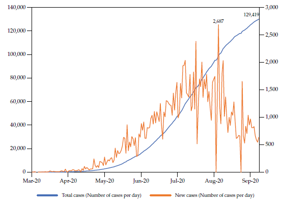
Source: Based on data from Mathieu et al. (2020) by Our World in Data.
The lockdown measures resulted in a negative shock in both demand and supply. In terms of aggregate supply, private firms' marginal productivity of the labor force was affected due to transportation restrictions and a portion of their workers getting infected. Moreover, the restrictions on land and air borders had a negative impact on goods imported for firms. The lockdown decreased the population's consumption and aggregate demand. In addition, the decrease in economic activity and the restrictions applied to companies caused a significant reduction in the private businesses' generated income.
In this way, economic activity quickly declined. As can be seen in Figure 2, the variation in the same period in the General Index of Economic Activity (IGAE) was negative twice: 1) during November 2019, as a product of social and political conflicts, and 2) between March and June 2020, as a result of the implementation of the lockdown.
Figure 2
Variation to the Same Period in igae, January 2018-June 2020 (in percent)
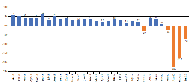
Source: Based on the National Institute of Statistics of Bolivia data.
During the first quarter of 2020, there was a slowdown in economic activity of only 0.5 % in the cumulative growth rate for those months -the lowest economic growth rate since the beginning of the twenty-first century. During the second quarter, the economic contraction deepened even further. In addition to the consequences of the lockdown, a historic fall in oil and commodity prices should be noted, further weakening economic activity and deepening the government's tax revenues recession.
The national economy experienced a decline, and most economic activities showed considerable negative growth rates (Figure 3). The most contracted economic activities were construction, transportation, and mining. However, it cannot be considered a generalized effect, given that activities such as agriculture, communications, and public administration services grew.
Figure 3
Variation to the same period in IGAE by economic activity, June 2020

(in percent)
(1) Includes the activities of restaurants and hotels; communal, social and personal; and domestic services.
Source: Based on National Institute of Statistics of Bolivia data.
Due to this economic scenario, Bolivia's unemployment rate increased since March 2020. As of July 2020, 11.8 %> of Bolivia's economically active population was unemployed (Figure 4). This employment behavior is in line with other countries in the region.
Figure 4
Bolivia’s Unemployment rate, January 2018-July 2020 (in percentage)
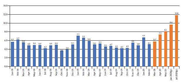
Source: Based on National Institute of Statistics of Bolivia data.
Two essential factors characterized Bolivia's 2020 public finances situation: 1) a decrease in tax revenue caused by the tax relief policies implemented and a decrease in economic activities due to the drastic reduction in mobility and trade among countries, and 2) an expansionary fiscal policy measures to counter the adverse economic effects of the Covid-19 pandemic.
As a result, in June 2020, Bolivia had a current fiscal deficit for the first time since 2004 (Figure 5), reaching a budget deficit of 12.7 % in relation to the GDP. On the other hand, the national public debt reached 19.4 billion dollars in the first months of 2020 (Figure 6) due to loans from international organizations and the Bolivian Central Bank to meet the needs generated by the health emergency. As of May 2020, the national public external debt in relation to the GDP reached 28.2 %, a number below the limit of 50 % recommended by the International Monetary Fund (IMF), which is a good indicator of debt sustainability.
Figure 5
Fiscal balance of Bolivia, 2000-June 2020
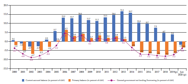
Source: Based on the Bolivia’s Ministry of Economy and Public Finance data.
Figure 6
National Public Debt of Bolivia, 2000-June 2020
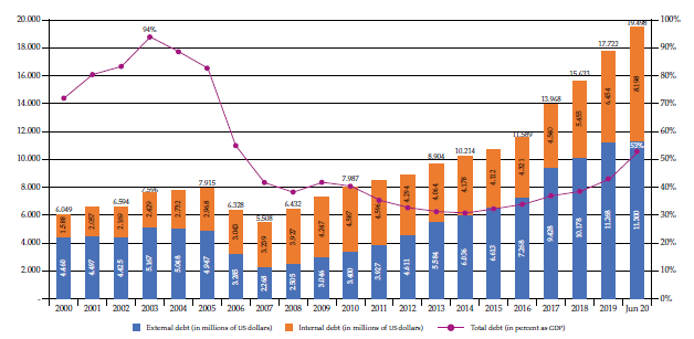
Source: Based on Bolivia’s Ministry of Economy and Public Finance data.
In general, the pandemic affected the deterioration of the national economy, the deterioration of sectoral economic activity, unemployment, and other macroeconomic variables, but the effects at the regional level have not been quantified.
2.2. Stylized fact of economic growth by region in Bolivia
Figure 7 reflects the effects before the pandemic. Thus, before it, the real GDP growth of Santa Cruz was the highest compared to the other departments followed by La Paz and Beni, with a growth of 4.15 %, 3.21 %, and 3.09 %, respectively for 2019.
Figure 7
Economic Growth by Region in Bolivia, 2000-2019 (in percentage)
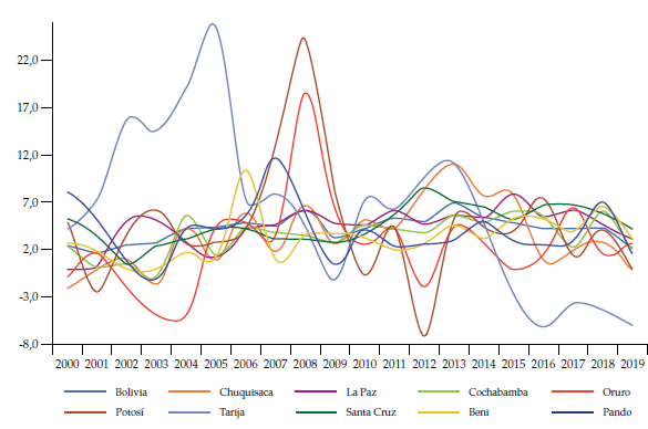
Source: Based on National Institute of Statistics of Bolivia data.
On the other hand, the annual GDP growth, in general, presents an erratic behavior for all departments, leaving aside Tarija, which presents a decreasing trend since 2013, due to its dependence on hydrocarbon production. It should be noted that only annual observations are available to measure the level of economic activity of the departments.
2.3. Economic Policy Measures in the Face of Covid-19 in Bolivia
To reactivate the economy, Bolivia's Ministry of Economy and Public Finance and the Central Bank designed and implemented an expansionary fiscal and monetary policy package. The following tables summarize the central economic policies performed in Bolivia.
Table 1
Main Monetary and Financial Policies Applied to Counteract the Economic Impact of Covid-19
Table 2
Main Fiscal Policies Applied to Counteract the Economic Impact of Covid-19
The three levels of government implemented measures to expand current and capital expenditure: central, regional, and main local governments. The central government contributed to the implementation and disbursement of direct cash transfers such as Bono Familia, Canasta Familiar and Bono Universal, basic services payment deferrals, and deferral, and extension of tax payment, among others, to guarantee income for Bolivian families. In addition, the government transferred resources from the NT to the local governments for prevention, containment, and treatment of the Covid-19 pandemic.
The expenditure plan for the NT in 2020 aimed at dealing with the national emergency and lockdown measures. It focused on strengthening the country's health system (purchasing of medical supplies and hiring healthcare personnel), mitigating the contraction of economic activity (increasing public spending and tax reliefs), and protecting the vulnerable population (providing cash transfers).
3. Methodology and Data
3.1. Mixed Frequency Multivariate Autoregressive Vectors with Stochastic Volatility
We aimed to quantify the economic performance by region in Bolivia (quarterly economic growth) to improve the regional economic policy design data. This study adopted an empirical model in line with the methodology of Koop et al. (2018) and applied it to Bolivia. We used a Mixed Frequency Multivariate VAR model with stochastic volatility (MF-VAR-SV) and a Bayesian method using the machine learning algorithm known as Dirichlet-Laplace Hierarchical.
The MF-VAR-SV model allows the estimation of high-frequency unobserved variables (quarterly, monthly, or daily) by simultaneously modeling the data of high-frequency not observed variables and low-frequency observed variables, subject to temporal and spatial restrictions. The Kalman filter is used to fill in missing observations.
Following Kim and Nelson (1999), the Kalman filter, initially developed by Kalman (1960), is a recursive process used to compute the optimal estimator of the unobserved component of a system, also called the state vector, at time t, based on the information available up to that period. The Kalman filter has a long history in different fields. For economics, the original developers were Sargent and Sims (1977) and Geweke and Singleton (1981), who began to use this filter through frequency domain methods. Then, Engle and Watson (1981) and Watson and Engle (1983) showed that these models could be estimated using maximum likelihood and state-space models, which allows for estimating the values of the latent factor using the Kalman filter.
To use the Kalman filter, one must express the dynamic system, including the unobserved variable, through a state-space model. State-space models consist of the transition equation and the measurement equation. The estimation of the model used the maximum likelihood method. The estimated coefficients were then adjusted using the Kalman filter algorithm. The following is the notation of the model in the state-space form:
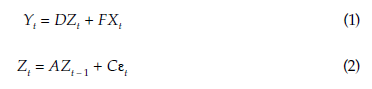
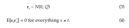
Where Z t is the vector containing the unobserved state variables, which in this context is the regional gdp, the error terms of the measurement equation, and their innovations; Y t is the vector containing the endogenous variables; X t is the vector containing the exogenous variables, and εt is a vector containing the error terms of the measurement equation.
Whereas F, A, and C are the matrix that contains the time-invariant parameters of the model. It is assumed that the error terms of the measurement equation have a normal distribution, with zero mean and no serial correlation:
Our model was constructed using the quarterly logarithmic variation of the gdp for Bolivia's r regions (r - 9) and transition and measurement equations. The transition equation seeks to estimate the quarterly indicator of economic activity for the nine regions of Bolivia (Y t Q ) using all the observable information available through the following var model:
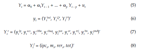
Where Y t is a vector of endogenous variables composed of three sets of variables:
-
Quarterly Real gpd (Yt bol), which is an observed variable.
-
Quarterly Regional Real gdp (Yt Q) which is a not observed variable. The regions were the following: La Paz (lp), Santa Cruz (scz), Cochabamba (cbba), Chuquisaca (chuq), Potosí (pot), Oruro (or), Tarija (trj), Beni (ben) and Pando (pnd).
-
Quarterly macroeconomic indicators observed in Bolivia relevant to a small and open economy: consumer price index (CPI), monetary aggregate m2 (m), the real exchange rate (RER), and terms of trade (TOT).
All variables are in logarithmic differences with one period lag. We used Census-13 seasonal adjustment to all variables. The sample ranges from the first quarter of 2001 to the second quarter of 2020. In the second quarter of 2020, we used the IGAE variation as a proxy of the quarterly GDP variation, which was the indicator available at that time. Although it is a sample that could be considered small, our analysis period is restricted by the availability of fiscal information. As will be seen in the following sections, we used disaggregated information on current and capital expenditure for central, regional, and main local governments that we could only obtain from the year 2000. We want to point out that this is an unprecedented database that was possible to build thanks to close collaboration with the Ministry of Economy of Bolivia, to which we send our thanks.
The elements Y t , are all observable and measurable except for the vector Y t Q . In addition, u t is the error of the estimation in equation (5), which is assumed to be independent and identically distributed with a distribution N(0, Σt).
We adopted a popular multivariate stochastic volatility specification (see Cogley and Sargent, 2005; Carriero et al., 2015). It decomposes the covari-ance matrix of the error as:
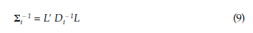
Where L is a lower triangular matrix and the diagonal D t is formed by the volatilities, which follow a random walk.
As it is well known, most empirical macroeconomic applications present evidence of changes in volatility. However, there is a tendency in mixed-frequency VAR literature to ignore this issue and work with homoscedastic models. As can be seen in Koop et al. (2018), which is the working paper version of Koop et al (2020), there is evidence in support of the use of this kind of MF-VAR-SV, because marginal likelihoods strongly indicated that stochastic volatility is present in real and nominal data.
We performed a robustness check using two quarterly exogenous variables per region: supermarket sales and consumption of concrete. The results from this exercise are not qualitatively different from the original specification. Given they restrict the sample, we did not use them for the rest of the document's analyses. They are available upon request to the users.
In line with Koop et al. (2018), Mariano and Murasawa (2003, 2010), Mitchell et al. (2005), and Schorfheide and Song (2015), the following mixed temporal frequency restriction was used:

Equation (10) is a restriction relating the endogenous variable observed at a regional level to the weighted sum of quarterly latent states. Specifically, it holds the relationship between the annual gdp growth rate (Y t r - A ) and the quarterly growth rate (Y r t ,Y r t-1 ,...,Y r t-6 ) for each region. In this way, we established a restriction between the annual frequency time series (Y t r,A ) and the quarterly frequency (Yt r), both expressed in logarithmic differences. This condition maintains the linear structure of the space state model. Note that (10) shows an approximate relationship between the annual and quarterly log differences. It does not represent the econometric specification but is a way to match quarterly and yearly growth rates.
To apply the restriction imposed in equation (10) to each of the country's regions, equation (11) was constructed:
The vector Y t A contains the annual regional gdp growth rates and is mathematically represented as:
In equation (11), M t A - 1. The matrix Ω A represents the numerical time constraints explained in equation (10), as presented in Koop et al. (2020). So, equation (11) links our quarterly regional data with the unobserved regional quarterly growth rates we wanted to estimate.
The vector z t is a matrix composed of 6 column vectors with the respective quarterly lags expressed in (7) for each region. Therefore, z t is defined as:

In addition, two restrictions were introduced for the country's GDP:

with µt ~ N(0,σcs 2 ).
This last equation represents the transversal restriction we imposed, which dictates the sum of the regional GDP to be equal to the national GDP. The derivation of this equation, using data on logarithmic differences, can be found in Mitchell et al. (2005).
We resolved the notorious over-parametrization problem of the proposed VAR with a Bayesian estimation method and selected priors values using the Dirichlet-Laplace Hierarchical algorithm (Bhattacharya et al. 2015). In this model, the variance priors determine the degree of contraction of the coefficient matrix.
The state equations for our state space model can be written in multi-variate regression form, where β = vec([Φ 0 , Φ 1 , …, Φ p ]′) is a k-dimensional vector of var coefficients. We define ß = (ß1, ..., ß k )', then the priors of each coefficient are independent:

Note that this prior would shrink the estimate of ß j towards the prior mean of zero relatives to a maximum likelihood estimate (mle). The prior variance, ψ k β υ2 j ,β 2 ,τβ 2 determines the degree of shrinkage. Large values of variance priors imply a tiny contraction, and the Bayesian estimate is similar to that of maximum likelihood. However, if the variance priors are close to zero, the coefficient becomes zero, and the corresponding variable is removed from the model.
The determining factors of the previous variance priors were treated as unknown parameters
and estimates. Therefore, the algorithm automatically decided whether these variance
priors should be close to zero. The Dirichlet-Laplace priors were hierarchically chosen
because they are expressed in unknown parameters requiring their priors. They involve
only one prior hyperparameter αß. Bhattacharya et al. (2015) recommended setting it to
The previous explanation regards the reduction of the MF-VAR coefficients matrix, but the Dirichlet-Laplace algorithm also chooses the coefficients of the covariances matrix for the error. Empirical evidence shows that this type of previous reduction in a high-dimensional parameters vector may help induce parsimony in a model (see Park and Casella, 2008). This model led to a posterior approximating to true value at a theoretically optimal rate, superior to other alternatives such as the Bayesian Lasso.
3.2. Time-Varying Parameter Vector Autoregressions
Time-varying parameter vector autoregressions (TVP-VAR) have become widely used to analyze macroeconomic time series behavior. Chan and Eisenstat (2018) found that TVP-VAR with stochastic volatility works better than a VAR of constant coefficients for macroeconomic modeling. TVP-VARS often include stochastic volatility (sv), which allows variation over time in the variations in error processes affecting VAR. Thus, the method intended to capture the data's temporal variation using a parsimonious but flexible model as in the VAR. Generally, it works within a flexible framework with random time variation for a wide range of non-linear behaviors in the data. Following Cogley and Sargent (2001), a substantial part of the literature opted for a flexible specification that can be used for many temporal variation patterns.
Unlike the fixed coefficient version of the VAR, the intersection parameters and the matrix of lags are allowed to vary over time in a prescribed manner (Lubik & Matthes, 2015). The TVP-VAR was specified as follows:
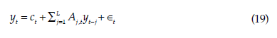
However, as the subscript t indicates, the intersection of direction and strength of autoregressive effects in (19) can take on different values over time.4 The lagged values were collected as follows: X′ t = I ∗ 1,′y t−1 …,y′ t−L ( ). θ t collects the var time variable coefficients in the vectorized form: θ t = vec, ([c t A 1 , t A 2 , t… A L, t ]′) which allowed us to rewrite the previous equation as follows:
The commonly assumed law of motion for θ t is a random walk:
Where µi ~ N(0, Q) is assumed to be independent of εt. The random walk specification is parsimonious because it can capture many patterns without introducing additional parameters. This assumption is primarily for parsimony and flexibility.
4. Results
This section presents the empirical results based on the methodologies indicated previously.
4.1. Analysis of the region's economic slowdown in Bolivia
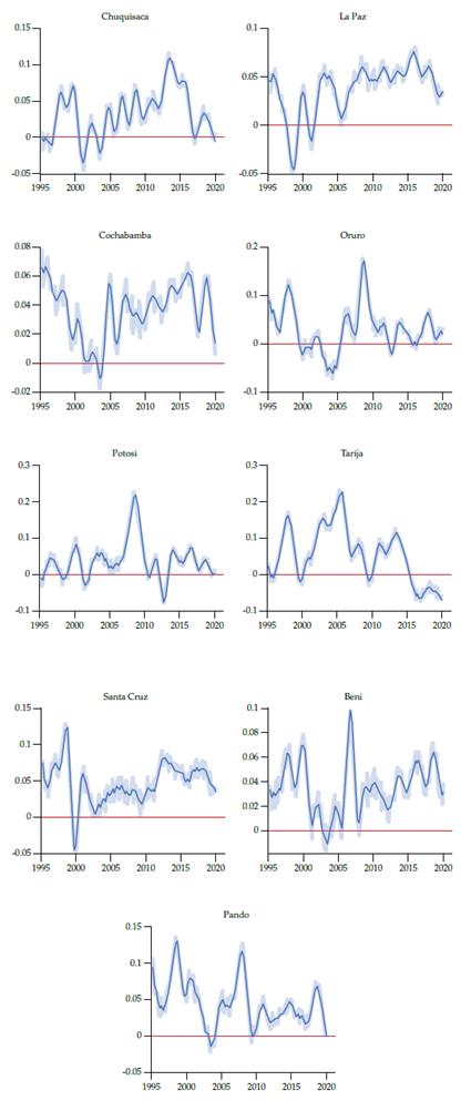
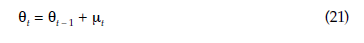
We present the estimated series of quarterly growth rates for the nine regions from the second quarter of 2000 to the second quarter of 2020 and a robustness check using an alternative specification with two exogenous variables -supermarket sales and concrete consumption in each region (Figures 8, 9 and 10). The graph shows that both series behave consistently. To convince the reader that our estimation produced accurate results, we present a plot with annualized quarterly economic growth (calculated using equation 10) by region, along with credible intervals which cover the 16th through 84th percentiles in annex B.
Figure 8
Seasonally Adjusted Quarterly Economic Growth by the Andean Region, 2000Q2-2020Q2 (in percentage)
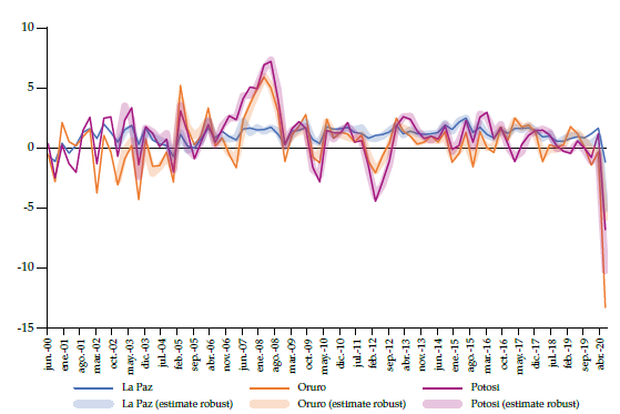
Source:
Figure 9
Seasonally Adjusted Quarterly Economic Growth by the Sub-Andean Region, 2000Q2-2020Q2 (in percentage)
Source:
Figure 10
Seasonally Adjusted Quarterly Economic Growth by the Llanos Region, 2000Q2-2020Q2 (in percentage)
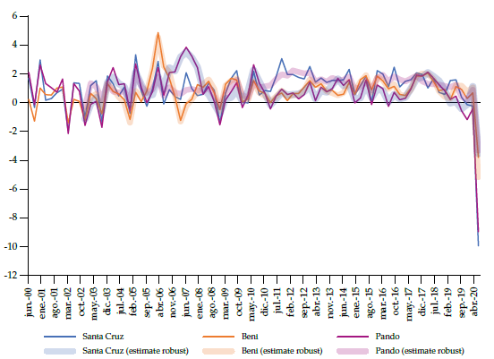
Source:
The pandemic and the confinement of economic activity, through the ex-post situation, allowed to appreciate a decrease of 7.2 % in national production as of June 2020 (National Institute of Statistics). Therefore, Table 3 also displays the seasonally adjusted quarterly growth rate by region for the last four quarters.
Table 3
Seasonally Adjusted Quarterly Growth rate by Region, 2019Q2-2020Q2 (in percentage)
The results show that the negative impact differed for each region, with Tarija, Oruro, Santa Cruz, and Pando being the most affected. In addition, from Figure 7, it can be deduced that the economic behavior is quite heterogeneous among regions, an example being Tarija, with a complicated economic situation since 2014, while others remained in a stable growth path at least until the second quarter of 2019.
4.2. Fiscal Policy Impact and Effectiveness Evaluation during Covid-19
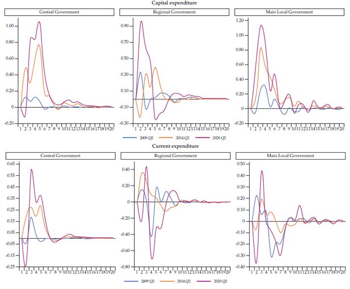
Through the TVP-VAR models, we can appreciate that during the second quarter of 2020, the growth rate of the nine regions responded positively to the shocks of capital expenditure of the central government. Chuquisaca, La Paz, and Beni reacted positively to regional government capital expenditure shocks, while Santa Cruz, Chuquisaca, and La Paz responded positively to capital expenditure shocks made by main local governments (Table 4).
Table 4
Growth Rate Response of Growth Rate to Capital and Current Expenditure Shocks (Second Quarter of 2020)
On the other hand, there is evidence that the regional growth rate did not respond to current expenditure shocks from regional and main local governments. However, Chuquisaca, Cochabamba, and Oruro's growth rates reacted positively to the current expenditure shocks of the central government.
To summarize, we noted that during the Covid-19 pandemic, central government capital spending was the most effective mechanism to mitigate the economic slowdown. We also identified that the response of economic activity to central government capital spending in the second quarter of 2020 was similar to that of the second quarter of 2009 and 2014 (time of economic slowdowns). Still, the magnitude of the former was much more significant (evidenced in annex B).
Finally, as a robustness check, we also made estimations using the variables of regional economic activity (supermarket sales and concrete consumption) following Koop et al. (2020). The results were consistent and very similar (see Figures 8, 9 and 10).
Conclusions
This research evaluates the role of fiscal policies applied in Bolivia to counteract the economic slowdown during the Covid-19 pandemic at a regional level. In general, it can be noted that the effects of the pandemic on economic growth at the regional level show a wide heterogeneity and depth of the impact, also, it must be considered that the speed of recovery will depend on each region's economic structure.
A Bayesian model of Mixed Frequency VAR with stochastic volatility (MF-VAR-SV) was estimated to construct a time series that represented the quarterly GDP growth rate for Bolivia's nine regions. In this way, we observed the country's regional GDP behavior. The results show that the negative impact on economic activity has been highly heterogeneous among the regions.
Later we assessed the effectiveness of fiscal policy during the pandemic. We estimated time-varying parameter vector autoregressions (TVP-VAR). The results show that the growth rate responded positively to central government capital spending shocks in most regions analyzed.
The model presented some limitations because the quarterly regional growth rates used are estimations, which can raise the difficulty of future predictability. Therefore, each region's sector effects (by economic activity) could not be obtained. For future research, we plan to analyze the level of regional cyclical synchronization since, in a scenario of economic contraction, it is essential to consider the economic synchronization of the different regions to find the most convenient economic policy.
Finally, we consider that high heterogeneity in regional economic growth has an implication for public policies. Policymakers should consider carrying out public policies differentiated by region to counteract economic recessions based on the optimal use of resources and the depth of economic contractions presented in each region. Our recommendation is in line with the administrative decentralization occurring in the country in recent years.